Workflow overview

This guide can help you start working with the Cadbiom command line.

Workflow for the Cadbiom framework. Four steps can be identified: Model building, covered by the standalone tool named biopax2cadbiom; Assisted query reconstruction, Causality search, Analysis and visualisation covered by the Cadbiom package named cadbiom-cmd.

The analysis of a BioPAX model is performed according to four main steps.

The first step of the Cadbiom framework relies on the biopax2cadbiom package. It allows querying BioPAX ontologies stored in public or local endpoints in order to interpret them into Cadbiom models.

The results of the conversions of some databases are available below: Characteristics of biopax ressources.

The second step brings together several commands under the name of query design. This step is dedicated to query construction. A query is a boolean logical formula that describes the combination of molecules for which regulators will be searched.

The characteristics of a Cadbiom model and its content (list of identifiers of biological compounds, list of boundary compounds, and list of genes) can be exported. Among the essential data, the user will find mappings between various databases thanks to the preservation of all cross-references with public databases (such as HGCN, Uniprot, Chebi) provided in the BioPAX. Indeed, Cadbiom uses internal identifiers to guarantee the uniqueness of the biomolecules in its models. A mapping of Cadbiom identifiers with the standard database identifiers is necessary to allow a user to build queries.

Examples of commands are described below: Query the Cadbiom model.

The third step of the workflow is focused on causality search. In this step, the user explores the dynamics of a Cadbiom model. He identifies sets of biomolecules that represent the initial conditions of the system, leading to the activation of the desired entities via controlled biochemical transformations described in the model. As detailed in the results section, the notion of activation is intrinsically linked to the non-deterministic semantics associated with guarded transitions. This analysis therefore generates several families of controllers associated with trajectories composed by the entities activated during a search.

Examples of commands are described below: Search for molecules.

The fourth step, visualization and analysis is designed to analyze the families of controllers generated in the previous step. A matrix of occurrences details the presence of controllers in the solutions obtained. Heatmaps allow estimating the diversity of the trajectories leading to the studied phenotype (i.e. the boolean query). Trajectory graphs allow visualizing all the transformations undergone by the intermediate molecules from the control molecules to the target molecules.

Examples of commands are described below: Processing of the generated files.

Characteristics of biopax ressources

The majority of models are pre-generated from the PathwayCommons archive and are made available on this page with their respective characteristics.

ACSN maps are preprocessed before there interrogation as RDF data. The maps are downloadable on acsn.curie.fr. The steps are explained on the GitLab.

Advanced users will be able to create their own models from a SPARQL endpoint as explained in the chapter Creation of a Cadbiom model from a BioPAX endpoint.

Obtaining these data from the models is also explained in the chapter Query the Cadbiom model.

Here is a table of the number of the BioPAX types found in various databases:

Metrics - Databases	PID	Kegg	ACSN
Entity			27426*
Pathway	745	122	13
Gene
PhysicalEntity			0/11922*
Protein	6194	1872	6851
Complex	4137		2323/2358*
SmallMolecule	173	1664	554/0*
Dna			1030
Rna	22		1164/0*
Interaction
BiochemicalReaction	1824	1782	6863
ComplexAssembly	2722		1743
TemplateReaction	1492
Transport	312		699
MolecularInteraction		4
Degradation
TransportWithBiochemicalReaction	154
Catalysis	3800	1782	6186
Control	322
TemplateReactionRegulation	2023
Modulation

*: Number before cleaning of incorrect/duplicate types in triplestore. i.e. the entire database, for the Entity type.

Here is a table presenting some metrics interpreted according to the raw BioPAX data obtained:

Metrics - Databases	PID	Kegg	ACSN
Retrieved PhysicalEntities	10526	3536	1716
Total of duplicated entities	699	135	74
Nb of groups of duplicated entities	339	61	23
Classes	403	0	0
Used classes	304	0	0
Nested classes	23	0	0
Classes with ModificationFeatures	157	0	0
Classes/complexes	66	0	0
Final number of entities (after processing)
Retrieved Reactions	6504	1786	9305
Proteins involved as reactants	3304	0	4840
SmallMolecules involved as reactants	128	1571	NA
Complexes involved as reactants	3733	0	2217
Retrieved Controls	6145	1782	6186
Catalysis control	3800	1782	494
Reactions with similar entities as reactants and products	50	934	333
Controls of other controls	0	0	0

Prebuilt models

Here is the the characteristics of the generated models:

Metrics - Databases	PID	Kegg	ACSN
Cadbiom entities	9788	2604	10313
Genes	788	2	1035
	csv/json	csv/json	csv/json
Boundaries	3925	1420	3693
	csv/json	csv/json	csv/json
Transitions	11036	5220	11394
Events	7501	1570	8819
Models	bcx file	bcx file	bcx file

Note: Use “Save as” after a right click on the download links if your browser tries to open files in a new tab…

Query the Cadbiom model

What is in the model?

As mentioned above, a user can either build his own model from any triplestore hosting BioPAX data, or use one of the pre-designed models provided earlier on this page.

He can then browse these models to extract data about all biomolecules, genes or boundaries (elements at the periphery of the model). Among the essential data, the user will find lists of mappings between various databases.

Indeed, Cadbiom uses internal identifiers to guarantee the unicity of biomolecules in its models. A mapping of the Cadbiom identifiers with the standard database identifiers (such as Uniprot, HUGO, etc.) is then necessary to allow the user to forge his own requests of interest (for more information on the search for molecules, see the next chapter: Search for molecules). This often tedious mapping step is facilitated by the module described below: Get a mapping between Cadbiom identifiers and those from external databases.

Get model information

To get information about the biological entities in the model, the subcommand model_info can be used (see the documentation of the model_info command) :

$ cadbiom_cmd model_info model_without_scc.bcx --all_entities --json --csv

Arguments:

• --all_entities or --boundaries or --genes: Retrieve data for specific places/entities of the model.
• --json: Create a JSON formated file containing data about previously filtered places/entities of the model, and a full summary about the model itself (boundaries, transitions, events, entities locations, entities types).
• --csv: Create a CSV file containing data about previously filtered places/entities of the model.

Example of JSON file for PID (model_summary_genes_pid.json):

{
    'modelFile': 'string',
    'modelName': 'string',
    'events': int,
    'entities': int,
    'boundaries': int,
    'transitions': int,
    'entitiesLocations': {
        'cellular_compartment_a': int,
        'cellular_compartment_b': int,
        ...
    },
    'entitiesTypes': {
        'biological_type_a': int,
        'biological_type_b': int;
        ...
    },
    'entitiesData': {
        [{
            'cadbiomName': 'string',
            'immediateSuccessors': ['string', ...],
            'uri': 'string',
            'entityType': 'string',
            'entityRef': 'string',
            'location': 'string',
            'names': ['string', ...],
            "xrefs": {
                'external_database_a': ['string', ...],
                'external_database_b': ['string', ...],
                ...
            }
        }],
        ...
    }
}

Such a file could facilitate a work of visualization or a possible mapping of identifiers because it centralizes in a standardized manner most of the information about BioPAX entities.

It can also be used to easily identify the entities of the model that we would like to remove in a future translation (Example: energy metabolism molecules such as ATP, ADP, GTP, GDP). Indeed, these molecules are ubiquitous and unnecessarily complexify the conditions of realization of the reactions in the model and thus its analysis by the solver.

Simplified example of CSV file (genes_pid.csv):

cadbiomName	immediateSuccessors	names	uri	entityType	location	uniprot knowledgebase	chebi
VCAM1_integral_to_membrane		VCAM1	Protein_xxx	Protein	integral to membrane	P19320
ATP	ADP	ATP	SmallMolecule_xxx	SmallMolecule			CHEBI:15422|CHEBI:22249

The most important field is probably `immediateSuccessors`, as it lists the immediate successors encountered for each entity in the model. This column contains the Cadbiom identifiers of entities that should be requested by a user who would like to explore their regulation with the framework. It is these identifiers that should constitute the queries (boolean logical formula) used in the Search for molecules section.

Get information about the graph based on the model

To build a graph based on the model and get information about it, the subcommand model_graph (see the documentation of the model_graph command) can be used:

$ cadbiom_cmd model_graph model_without_scc.bcx --graph --centralities --json

Arguments:

• --centralities: Get centralities for each node of the graph (degree, in_degree, out_degree, closeness, betweenness).
• --graph: Translate the model into a GraphML formated file which can be opened in Cytoscape.
• --json: Create a JSON formated file containing a summary of the graph based on the model.

Example of JSON file (graph_summary_pid.json):

{
    'modelFile': 'string',
    'modelName': 'string',
    'events': int,
    'entities': int,
    'transitions': int,
    'graph_nodes': int,
    'graph_edges': int,
    'centralities': {
        'degree': {
            'entity_1': float,
            'entity_2': float
        },
        'in_degree': {
            'entity_1': float,
            'entity_2': float
        },
        'out_degree': {
            'entity_1': float,
            'entity_2': float
        },
        'betweenness': {
            'entity_1': float,
            'entity_2': float
        },
        'closeness': {
            'entity_1': float,
            'entity_2': float
        },
    }
}

The corresponding GraphML file can be downloaded here pid.graphml.

Examples of use and style dedicated to opening the GraphML file in Cytoscape are available on the repository: examples

Also a dedicated a module dedicated to viewing the models in Gephi is also available as explained later.

Get a mapping between Cadbiom identifiers and those from external databases

This function exports a CSV formated file presenting the list of known Cadbiom identifiers for each given external identifier.

$ cadbiom_cmd identifiers_mapping --external_identifiers P02452 COL1A1 P12830 CDH1 model_pid_without_scc.bcx

Arguments:

• --external_identifiers: Multiple external identifiers to be mapped.

Example of CSV file (mapping.csv):

External identifiers	Cadbiom identifiers
P12830	E_cadherin_early_endosome|E_cadherin_cytoplasm|E_cadherin_gene|…
CDH1	E_cadherin_early_endosome|E_cadherin_cytoplasm|E_cadherin_gene|…
P02452	COL1A1_gene|COL1A1
COL1A1	COL1A1_gene|COL1A1

Search for molecules

With a given model, Cadbiom allows to explain how to obtain an entity or a set of entities from boundaries (elements at the periphery of the model). These sets are called Minimal Activation Conditions (MAC).

Ultimately, the software answers to the question: “Is it possible to find an initialization such that the given state/property happens?”

Searching a complex query with a combination of entities requires to express it in a boolean formula with the names of the entities as variables. The logical operators available are or, and, not.

See the section Get model information in order to find out which entities to query in the model.

The subcommand solutions_search is designed to compute MACs.

Example:

We are looking for entities involved in the production of extracellular matrix molecules. Some combinations of these entities are gathered in the following file: logical_formulas.txt.

This file is then loaded in the solver with the following command:

$ cadbiom_cmd solutions_search model_without_scc.bcx --input_file logical_formulas.txt --continue

Arguments:

Most of the time, the number of steps to reach a solution is significant and therefore, the necessary computation time ensues. Fortunately, it can be limited with --steps. Moreover, a stopped calculation can be resumed later thanks to --continue.

• --input_file: Multiple jobs can be launched in parallel if the user provides a file with one boolean formula per line. In this case, each processor core will be dedicated to the calculation of one boolean formula (within the limit of the number of available cores).

• --continue: Resume previous computations; if there is a mac file from a previous work, last frontier places/boundaries will be reloaded.

—

The program produces two categories of files; a quick description is provided here but for further information please see chapter Cadbiom File Format Specification):

• *mac.txt files: Each line contains a MAC solution. Here is an example taken from the file corresponding to the query COL1A1 and COL3A1 and COL5A1 and MMP2 and not PERP (Mac file).

  COL1A1_gene COL3A1_gene COL5A1_gene dNp63a__tetramer__nucleus_v2 ET1_extracellular_region ETA FOXM1B_nucleus GTF3A MMP2_gene
  COL1A1_gene COL3A1_gene COL5A1_gene dNp63a__tetramer__nucleus_v2 ET1_extracellular_region ETA Fra1_1O_2O_nucleus GTF3A JUN_2O_2O_nucleus MMP2_gene
  

• *mac_complete.txt files: Each MAC solution is followed by the successions of events fired at each step to obtain them. Here is an example taken from the file corresponding to the query COL1A1 and COL3A1 and COL5A1 and MMP2 and not PERP (Mac complete file).

  COL1A1_gene COL3A1_gene COL5A1_gene dNp63a__tetramer__nucleus_v2 ET1_extracellular_region ETA FOXM1B_nucleus GTF3A MMP2_gene
  % _h_5848 _h_1070 _h_4563 _h_4049
  % _h_5603 _h_1051
  COL1A1_gene COL3A1_gene COL5A1_gene dNp63a__tetramer__nucleus_v2 ET1_extracellular_region ETA Fra1_1O_2O_nucleus GTF3A JUN_2O_2O_nucleus MMP2_gene
  % _h_5848 _h_1070 _h_4283
  % _h_4174 _h_4049 _h_1051
  

As we can see, these files are not particularly meaningful, which is why the next chapter Processing of the generated files will discuss how to use the high-level features available to handle them.

Processing of the generated files

Visualize the trajectories of each solution

In the same way that we can generate a graph of the model, we can generate a graph explaining the path taken for each solution found by the solver. We are therefore reconstructing the path between boundaries of the model (the components of the solutions) and entities of interest in order to explain their production.

This command requires the model and solution files of type *.mac_complete.txt. We will take the example of the file seen in the previous chapter.

Example:

$ cadbiom_cmd solutions_2_graph model_without_scc.bcx \
  "./result/model_without_scc_COL1A1 and COL3A1 and COL5A1 and MMP2 and not PERP_mac_complete.txt"

—

The program produces GraphML files in the folder ./graphs/. These files can be opened in Cytoscape.

Cytoscape screenshot of the graph of the first solution for the query COL1A1 and COL3A1 and COL5A1 and MMP2 and not PERP.

Cytoscape screenshot of the graph of the second solution for the query COL1A1 and COL3A1 and COL5A1 and MMP2 and not PERP.

We notice that the paths taken are relatively similar and independent for each of the 4 entities searched (4 cliques are displayed). However, the solver has found an alternative path to the first solution in order to produce MMP2.

The more solutions listed, the more complex they become and require different boundaries. We also note that the reactions most described in the literature such as the translation of the MMP2 gene are the most likely to have a significant number of referenced modulators. It is around these reactions that the complexity of the model is revealed.

Cytoscape screenshot of the graph of the 343rd solution for the query COL1A1 and COL3A1 and COL5A1 and MMP2 and not PERP.

Global visualization of all paths found for a query

solutions_2_common_graph

Create a GraphML formated file containing a unique representation of all trajectories corresponding to all solutions in each complete MAC file (*mac_complete files). This is a function to visualize paths taken by the solver from the boundaries to the entities of interest.

Example:

$ cadbiom_cmd queries_2_common_graph model_without_scc.bcx \
  "./result/model_without_scc_COL1A1 and COL3A1 and COL5A1 and MMP2 and not PERP_mac_complete.txt"

Generated graph (graph):

Cytoscape screenshot of common weighted and directed graph of solutions for the query COL1A1 and COL3A1 and COL5A1 and MMP2 and not PERP.

Programmatic processing and decompilation of solution files

queries_2_json

Create a JSON formated file containing all data from complete MAC files (*mac_complete files). The file will contain frontier places/boundaries and decompiled steps with their respective events for each solution. This is a function to quickly search all transition attributes involved in a solution.

Example:

$ cadbiom_cmd solutions_2_json model_without_scc.bcx \
  "./result/model_without_scc_COL1A1 and COL3A1 and COL5A1 and MMP2 and not PERP_mac_complete.txt"

Example of JSON file (decompiled_mac_complete):

[{
    "solution": "boundary_1 boundary_2",
    "steps": [
        [{
            "event": "_h_1",
            "transitions": [{
                "ext": "place_x",
                "ori": "boundary_1"
            }]
        }],
    ]
},
...
]

Search of interactions between molecules in trajectories

Search of interactions between molecules present in the trajectories and the boundaries with distinction of genes and various stimuli (non genes).

json_2_interaction_graph

Make an interaction weighted graph based on the searched molecule of interest. Read decompiled solutions files (.json files produced by the directive ‘solutions_2_json’) and make a graph of the relationships between one or more molecules of interest, the genes and other frontier places/boundaries found among all the solutions.

Example:

$ cadbiom_cmd json_2_interaction_graph model_without_scc.bcx \
  "./decompiled_solutions/model_without_scc_COL1A1 and COL3A1 and COL5A1 and MMP2 and not PERP_mac_complete_decomp.json" \
  PKC_1a
INFO: Opening files...
INFO: Files processed: 1
INFO: Building graph...
INFO: Graph generated in 0.0767540931702

Generated graph (interaction graph between PKC_1a and boundaries):

Cytoscape screenshot of the interaction graph of the entity PKC_1a for the query COL1A1 and COL3A1 and COL5A1 and MMP2 and not PERP.

Occurrences matrix

solutions_2_occcurrences_matrix

Create a matrix of occurrences counting entities in the solutions found in *mac.txt files in the given path.

Example:

$ cadbiom_cmd solutions_2_occcurrences_matrix output/pid_last_nov_model_without_scc.bcx \
  ./result/ \
INFO: Files processed: 44

occurrences matrix transposed occurrences matrix

Clustermaps

We can visualize co-occurrences of the boundaries within the solutions obtained by creating a ClusterMap (hierarchically-clustered heatmap) for boundaries found in the solutions.

Example:

$ cadbiom_cmd queries_2_clustermap \
  "./result/model_without_scc_COL1A1 and COL3A1 and COL5A1 and MMP2 and not PERP_mac_complete.txt"


pid_last_nov_model_without_scc_COL1A1 and COL3A1 and COL5A1 and MMP2 and not PERP_mac

Generated clustermap (clustermap.svg)

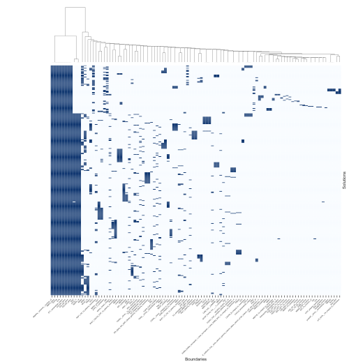
Hierarchically-clustered heatmap of the occurrences of the boundaries found in the solutions for the query COL1A1 and COL3A1 and COL5A1 and MMP2 and not PERP.

Avanced users - Creation of models

Creation of a Cadbiom model from a BioPAX endpoint

biopax2cadbiom is a standalone module also integrated in the Cadbiom GUI that converts BioPAX ontologies to Cabiom models. You will find a full help about the installation and usage at biopax2cadbiom. Do not miss the chapter How to make queries on an endpoint like Pathway Commons?

Let’s take the example of a PID database (Pathway Interaction Database) conversion with the following command:

$ biopax2cadbiom model \
--graph_uris http://pathwaycommons.org \
--provenance_uri http://pathwaycommons.org/pc2/pid \
--triplestore http://rdf.pathwaycommons.org/sparql/

Quick explanations of arguments:

• The parameter --graph_uris provides the URI of the graphs queried (and optionally of the BioPAX ontology if it is hosted separately).
• It is thus necessary to filter the RDF triples according to their origin with the the optional parameter --provenance_uri. By setting it, the program will filter entities, reactions, pathways thanks to their dataSource BioPAX attribute.
• The URL of the endpoint is specified with --triplestore.

Result:

The generated model will be placed in the ./output folder; we will focus on the model with specific alterations intended to optimize the operation of Cadbiom and its solver: ./output/model_without_scc.bcx.

(pid_model_without_scc.bcx)

Note

Small graphs can be queried and converted from the GUI of Cadbiom.

Screenshot of the import tool for BioPAX graphs in the GUI of Cadbiom.